
データセット raincloud を data に格納します(ファイルの読み込み)
使用するパケージ
R
library(ggplot2)
library(ggdist)
library(dplyr)
library(gridExtra)
描き方は、ChatGPTにプロンプトして教えてもらいました
Raincloud plotの作成
R
g1 <- ggplot(data, aes(x = group, y = value, fill = group)) +
  ggdist::stat_halfeye(
    adjust = 0.5,
    justification = -0.2,
    .width = 0,
    point_colour = NA
  ) +
  geom_boxplot(
    width = 0.12,
    outlier.shape = NA
  ) +
  ggdist::stat_dots(
    side = "left",
    justification = 1.1,
    dotsize = 0.7
  ) +
  theme_minimal() +
  coord_flip() # 図を左に90度回転
print(g1)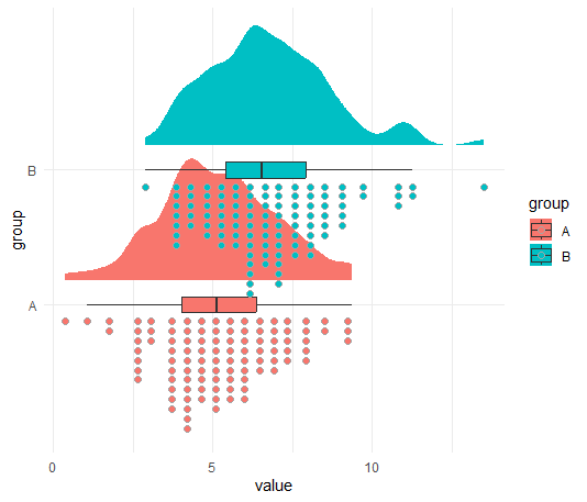
図Aと図Bを別に描いて間隔をあけます
R
# グループAのRaincloud plotの作成(オレンジ色)
plot_A <- ggplot(data %>% filter(group == "A"), aes(x = group, y = value, fill = group)) +
  ggdist::stat_halfeye(
    adjust = 0.5,
    justification = -0.2,
    .width = 0,
    point_colour = NA
  ) +
  geom_boxplot(
    width = 0.12,
    outlier.shape = NA
  ) +
  ggdist::stat_dots(
    side = "left",
    justification = 1.1,
    dotsize = 0.7
  ) +
  theme_minimal() +
  coord_flip() +
  scale_fill_manual(values = c("A" = "orange")) +
  scale_y_continuous(limits = c(0, 13), breaks = seq(0, 13, 1)) +
  labs(title = "Group A")

# グループBのRaincloud plotの作成(緑色)
plot_B <- ggplot(data %>% filter(group == "B"), aes(x = group, y = value, fill = group)) +
  ggdist::stat_halfeye(
    adjust = 0.5,
    justification = -0.2,
    .width = 0,
    point_colour = NA
  ) +
  geom_boxplot(
    width = 0.12,
    outlier.shape = NA
  ) +
  ggdist::stat_dots(
    side = "left",
    justification = 1.1,
    dotsize = 0.7
  ) +
  theme_minimal() +
  coord_flip() +
  scale_fill_manual(values = c("B" = "green")) +
  scale_y_continuous(limits = c(0, 13), breaks = seq(0, 13, 1)) +
  labs(title = "Group B")

# プロットの結合(縦に並べる)
grid.arrange(plot_A, plot_B, ncol = 1)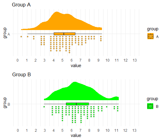
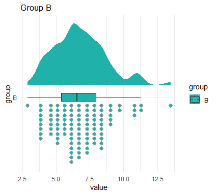
図Bのみを描く
R
# グループBのRaincloud plotの作成(緑色)
plot_B <- ggplot(data %>% filter(group == "B"), aes(x = group, y = value, fill = group)) +
  ggdist::stat_halfeye(
    adjust = 0.5,
    justification = -0.2,
    .width = 0,
    point_colour = NA
  ) +
  geom_boxplot(
    width = 0.12,
    outlier.shape = NA
  ) +
  ggdist::stat_dots(
    side = "left",
    justification = 1.1,
    dotsize = 0.7
  ) +
  theme_minimal() +
  coord_flip() +
  scale_fill_manual(values = c("B" = "#20B2AA")) +
  labs(title = "Group B")

# グループBのプロットを描画
print(plot_B)