

ターゲットが2値変数の場合
データの準備
Rをリセットしてデータreha_data.csvを再度読み込みます。
rm(list = ls(all.names = TRUE))
data <- read.csv("reha_data.csv", header=T, fileEncoding = "UTF-8")
head(data)
age sex preFIM duration postFIM
1 70 0 49 10 46
2 27 0 45 11 47
3 73 0 47 17 49
4 68 1 45 16 49
5 51 0 49 16 50
6 35 0 49 11 51使用するパッケージ(パッケージのインストール)
library(xgboost)
library(dplyr)
library(caret)
library(Matrix)ターゲットとなる変数(target)を作成します。ここでは、postFIMの中央値以上であれば1、未満であれば0となる2値変数を作成してdataに追加します。
median_postFIM <- median(data$postFIM, na.rm = TRUE)
data <- data %>%
    mutate(target = ifelse(postFIM >= median_postFIM, 1, 0))
table(data$target)
> table(data$target)
0 1
99 101 特徴量として必要な列だけを抽出したデータフレームを作成します。
df <- data %>% dplyr::select(age, sex, preFIM, duration, target)
head(df)
age sex preFIM duration target
1 70 0 49 10 0
2 27 0 45 11 0
3 73 0 47 17 0
4 68 1 45 16 0
5 51 0 49 16 0
6 35 0 49 11 0特徴量(x)とターゲット(y)に分離します。
x <- df %>% dplyr::select(-target)
head(x)
y <- df$target
head(y)
> x <- df %>% dplyr::select(-target)
> head(x)
age sex preFIM duration
1 70 0 49 10
2 27 0 45 11
3 73 0 47 17
4 68 1 45 16
5 51 0 49 16
6 35 0 49 11
> y <- df$target
> head(y)
[1] 0 0 0 0 0 0学習データ、テストデータ
createDataPartition関数によりデータセットを学習データ80%とテストデータ20%に分割します。
set.seed(123)
train_index <- createDataPartition(y, p = 0.8, list = FALSE)
x_train <- x[train_index, ]
x_test <- x[-train_index, ]
y_train <- y[train_index]
y_test <- y[-train_index]
学習データとテストデータからXGBoostモデルの入力形式に適合するデータ構造を作成します。
dtrain <- xgb.DMatrix(data = as.matrix(x_train), label = y_train)
dtest <- xgb.DMatrix(data = as.matrix(x_test), label = y_test)
XGBoostのパラメータ設定
XGBoostのパラメータを設定します。設定したパラメータをセットとしてparamsに格納します。
params <- list(
  objective = "binary:logistic",
  eval_metric = "logloss",
  max_depth = 3,
  eta = 0.1
)
学習データを使用した機械学習の実行
次に、XGBoostライブラリを用いてモデルの訓練を実行します。
model <- xgb.train(
  params = params,
  data = dtrain,
  nrounds = 100,
  watchlist = list(train = dtrain, eval = dtest),
  verbose = 0
  )
学習されたモデルによる予測
学習済みのXGBoostモデルを使って、テストデータに対する予測を行います。
pred_prob <- predict(model, as.matrix(x_test))
hist(pred_prob)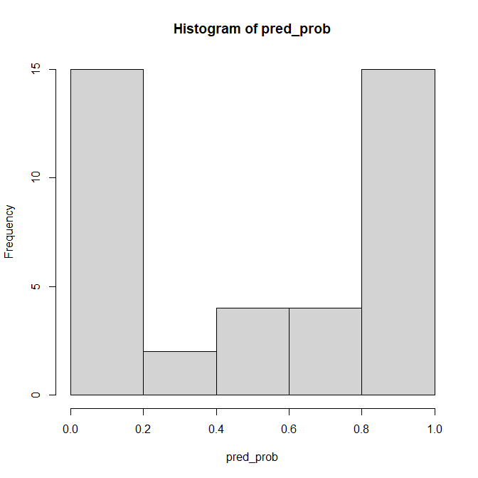
予測された確率は pred_prob という変数に保存されます。これにより、後で予測結果を分析したり、評価指標を計算したりする際に使用できます。このプログラムは、モデルの実用性をテストするための典型的なステップです。訓練されたモデルが実際にどのように機能するかを見るために、未知のデータ(この場合はx_test)に対する予測を行い、その予測の正確性や有用性を評価することができます。
as.matrix: テストデータを行列形式に変換します。XGBoost で使用する predict() 関数は、入力としてテストデータを 行列(matrix)または DMatrix 形式で渡す必要があります。モデルは objective = “binary:logistic” に基づく 二値分類タスクを解いており、各テストサンプルに対して 0〜1 の範囲の確率を出力します(そのサンプルが「1」である確率を示します)。
予測した確率を0.5を境に2値変数pred_labelに変換し、予測ラベル pred_labelとします。
pred_label <- ifelse(pred_prob >= 0.5, 1, 0)
table(pred_label)
pred_label
0 1
19 21 予測結果とテストデータを比較します(混同行列)。
confusionMatrix(
  data = factor(pred_label, levels = c("1", "0")),
  reference = factor(y_test, levels = c("1", "0"))
)
pred_label(予測された2値変数)と y_test(テストデータの2値変数)を比較し、混同行列(Confusion Matrix)を出力します。これにより、モデルの分類性能(正解率、感度、特異度など)を評価できます。
Confusion Matrix and Statistics

          Reference
Prediction  1  0
         1 18  3
         0  4 15

               Accuracy : 0.825
                 95% CI : (0.6722, 0.9266)
    No Information Rate : 0.55
    P-Value [Acc > NIR] : 0.0002476

                  Kappa : 0.6482

 Mcnemar's Test P-Value : 1.0000000

            Sensitivity : 0.8182
            Specificity : 0.8333
         Pos Pred Value : 0.8571
         Neg Pred Value : 0.7895
             Prevalence : 0.5500
         Detection Rate : 0.4500
   Detection Prevalence : 0.5250
      Balanced Accuracy : 0.8258

       'Positive' Class : 1
True Positive(TP): 18(実際も予測も1)
True Negative(TN): 15(実際も予測も0)
False Positive(FP): 3(実際は0だが予測は1)
False Negative(FN): 4(実際は1だが予測は0)
Accuracy : 全体のうち、正しく分類された割合。(TP + TN) / 全体。→ 82.5%の正解率。
Kappa : 偶然一致を考慮した一致率。0.6以上は「中等度以上の一致」とされる。モデルの妥当性が中〜高程度と判断できる。
Mcnemar’s Test P-Value : FPとFNの差に統計的有意差があるかを検定する。p値が高い(1.0)ため、誤分類に偏りはない=バランス良好。
Sensitivity : 実際に陽性(1)であるものを陽性と予測できた割合(= TP / (TP + FN))。→ 陽性を82%見逃さず検出できている。
Specificity : 実際に陰性(0)であるものを陰性と予測できた割合(= TN / (TN + FP))。→ 陰性を83%正しく検出できている。
Pos Pred Value : モデルが陽性と予測した中で、実際に陽性だった割合(= TP / (TP + FP))。→ 陽性予測のうち約86%が正解。
Neg Pred Value : モデルが陰性と予測した中で、実際に陰性だった割合(= TN / (TN + FN))。→ 陰性予測のうち約79%が正解。
Prevalence : 実際に陽性(1)だったデータの割合。→ データ全体の55%が陽性。
Detection Rate : 全体のうち、正しく陽性と予測された割合(= TP / 全体)。→ 全体の45%を正しく陽性と判定。
Detection Prevalence : モデルが陽性と判定した割合(= TP + FP / 全体)。→ 全体の52.5%が陽性と判定された。
Balanced Accuracy : 感度と特異度の平均値((Sensitivity + Specificity) / 2)。→ クラス不均衡の影響を受けにくい精度指標。
ROC曲線とAIC(赤池情報量規準)
XGBoostの性能を客観的・包括的に測るのが ROC曲線とAUC であり、これは確率出力を前提とした評価方法です。
ROC曲線を描画し、モデルの性能をAUC(曲線下面積)で評価します。XGBoostにはAICの直接的な定義がないため、比較としてロジスティック回帰を使い、AIC(赤池情報量規準)を算出します。AICはモデルの良さ(情報損失の少なさ)と複雑さのバランスを評価します。
# Add Libraries
library(pROC)    # For ROC curve and AUC
library(MASS)    # For AIC calculation (using general functions)

# Calculate ROC Curve and AUC
roc_obj <- roc(y_test, pred_prob)
auc_value <- auc(roc_obj)
ROC解析における roc() 関数では、
case= 陽性クラス(positive class)control= 陰性クラス(negative class)
として扱われます。
Setting levels: control = 0, case = 1
Setting direction: controls < cases
ROC曲線、AUC、AIC
# Plot ROC Curve
plot(roc_obj, col = "blue", main = sprintf("ROC Curve (AUC = %.3f)", auc_value))

# Alternative AIC calculation (since AIC is not directly defined for XGBoost, approximate using log-likelihood)
# Use logistic regression for comparison and calculate AIC
logit_model <- glm(target ~ age + sex + preFIM + duration, data = df, family = binomial)
aic_value <- AIC(logit_model)

# Display AUC and AIC
cat(sprintf("AUC: %.4f\n", auc_value))
cat(sprintf("AIC (Logistic Regression): %.2f\n", aic_value))
> cat(sprintf("AUC: %.4f\n", auc_value))
AUC: 0.9369
> cat(sprintf("AIC (Logistic Regression): %.2f\n", aic_value))
AIC (Logistic Regression): 99.27