

使用するパッケージ
R
library(pROC)
library(Epi)
データセット ROC をdata に読み込みます(ファイルの読み込み方)
dis: 罹患の有無(1=罹患, 0=健常)
test: 検査の点数 0, 1, 2, 3, 4(0は反応なし、4は反応あり)
このtestで罹患の有無を判断するためには、何点で陽性とするのがベターか?
R
head(data)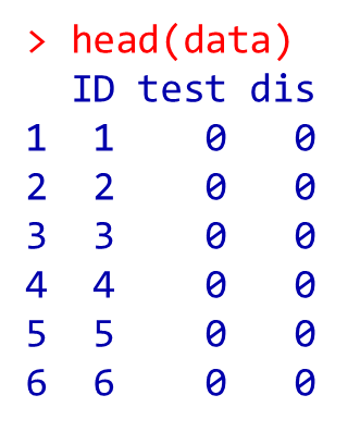
R
#変数disをファクターに変更(基準の変更が可能になります)
data$dis <- as.factor(data$dis)
#relevel関数で基準となるカテゴリーを設定します
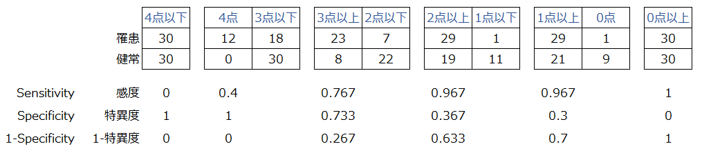
data$dis <- relevel(data$dis, ref="1") testの点数に該当する罹患者数
R
xtabs(~dis+test, data=data)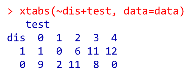
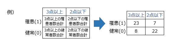
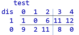
感度$=\frac{23}{23+7}=0.767$
特異度$=\frac{22}{8-22}=0.733$
この要領で全ての分割表から感度・特異度を算出します
この結果からROC(Receiver Operating Characteristic)曲線が描かれます
R
#感度
Sensitivity <- c(0, 0.4, 0.7667, 0.9667, 0.9667, 1)

#特異度
Specificity <- c(1, 1, 0.7333, 0.3667, 0.3, 0)

#1-特異度(偽陽性)
f_positive <- c(rep(1,6)) - c(1, 1, 0.7333, 0.3667, 0.3, 0)

#ROC曲線
plot(f_positive, Sensitivity, type="o", xlab="1-特異度", ylab="感度")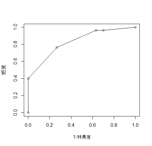
AUCと信頼区間
AUC(Area Under the Curve)は、ROC曲線の下の面積を指します。パッケージpROCの “roc関数” を使用することで、上述したROC曲線が出力されいます。
R
ROC <- pROC::roc(dis ~ test, data = data, ci = TRUE)
print(ROC)
R
plot(ROC)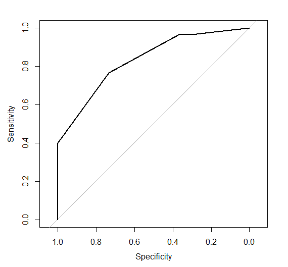
感度と特異度
もりとんroc関数の結果から感度、特異度も抽出できます
R
#感度
ROC$sensitivities

#特異度
ROC$specificities

#偽陽性
1 - ROC$specificities
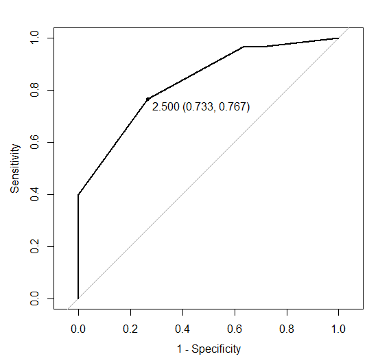
カットオフ値(yoden indexと左上隅からの最小距離)
R
plot(ROC,
    identity = TRUE,
    print.thres = "best",
    print.thres.best.method="youden", #closest.topleft=左上隅との距離が最小
    legacy.axes = TRUE
)
おまけ
R
data$dis <- relevel(data$dis, ref="0")
Epi::ROC(test=data$test, stat=data$dis, plot="ROC")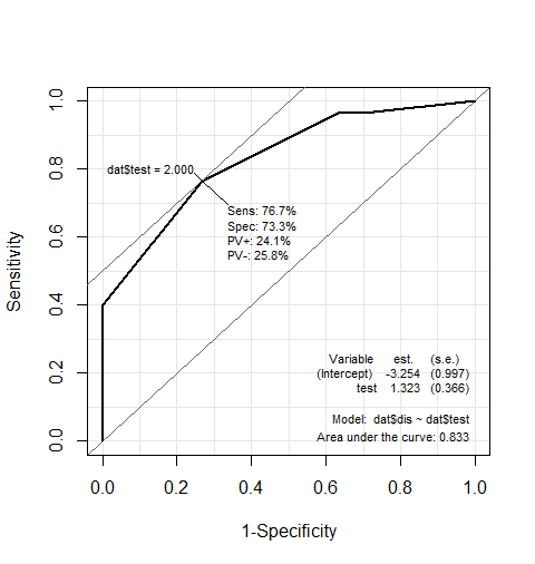
サンプルデータ
出典)柳川 堯 , 荒木 由布子; バイオ統計の基礎―医薬統計入門,近代科学社 ,2010,p12