

注意)乱数を使用しておりますので、微妙に異なる結果となります。
R
library(boot)

# Setting up the sample data
data <- c(5, 9, 8, 13, 6)

# Defining the bootstrap function
# Resample from the sample and calculate the mean
boot_mean <- function(data, indices) {
  sample_mean <- mean(data[indices])
  return(sample_mean)
}

# Calculating confidence intervals using the bootstrap method
boot_results <- boot(data, statistic = boot_mean, R = 500)
# Calculating the confidence intervals
boot_ci <- boot.ci(boot_results, type = "bca")

# Outputting the 95% confidence interval, rounded to two decimal places
cat("95% Confidence Interval: [",
    format(round(boot_ci$bca[4], 2), nsmall = 2), ", ",
    format(round(boot_ci$bca[5], 2), nsmall = 2),
    "]\n")

R
# Creating a scatter plot
plot(
  x = 1:500,
  y = boot_results$t,
  xlab = "Iteration",
  ylab = "Sample Mean",
  main = "Bootstrap Sample Means"
  )
# Drawing a horizontal line at the mean of the original data
abline(h = mean(data), col = "red", lwd = 2, lty = 2)
# Lower limit of the 95% confidence interval
abline(h = boot_ci$bca[4], col = "blue", lwd = 2, lty = 2)
# Upper limit of the 95% confidence interval
abline(h = boot_ci$bca[5], col = "blue", lwd = 2, lty = 2) 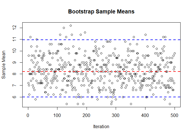
参考文献)坂巻顕太郎、篠崎智大(監修), 生物統計学の道標, 一般財団法人 厚生労働統計協会, 2023, p94